|
<< Click to Display Table of Contents >> radiative_boundary |
  
|
|
<< Click to Display Table of Contents >> radiative_boundary |
|
{ RADIATIVE_BOUNDARY.PDE
This example demonstrates the implementation of radiative heat loss
at the boundary of a heat transfer system.
}
title "Axi-symmetric Anisotropic Heatflow, Radiative Boundary"
select errlim=1.0e-4
coordinates { Define cylindrical coordinates with symmetry axis along "Y" } ycylinder("R","Z")
variables { Define Temp as the system variable, with approximate variation range of 1 } Temp(1)
definitions kr = 1 { radial conductivity } kz = 4 { axial conductivity }
{ define a Gaussian source density: } source = exp(-(r^2+(z-0.5)^2))
{ define the heat flux: } flux = vector(-kr*dr(Temp),-kz*dz(Temp))
initial values Temp = 1 |
|
equations { define the heatflow equation: }
Temp : div(flux) = Source
boundaries { define the problem domain }
Region 1 { ... only one region }
start "RAD" (0,0) { start at bottom on axis and name the boundary }
natural(temp)= 0.5*temp^4 { specify a T^4 boundary loss }
line to (0.5,0) { walk the boundary }
arc(center=0.5,0.5) angle 180 { a circular outer edge }
line to (0,1)
natural(temp)=0 { define a symmetry boundary at the axis }
line to close
monitors
elevation(magnitude(2*pi*r*flux)) on "RAD" as "Heat Flow"
contour(Temp) { show contour plots of solution in progress }
plots { write these hardcopy files at completion }
grid(r,z) { show final grid }
contour(Temp) { show solution }
surface(Temp)
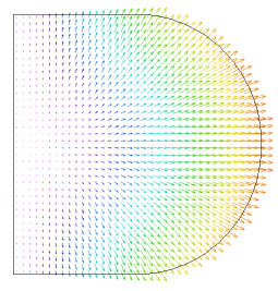
vector(2*pi*r*flux) as "Heat Flow"
elevation(magnitude(2*pi*r*flux)) on "RAD" as "Heat Flow" export
end